Calculus in MATLAB

Calculus is important in different fields like engineering, physics, and other sciences, but the calculations are done by machines or computers, whether they are into Physics or engineering. The tool used here is MATLAB, it is a programming language used by engineers and scientists for data analysis. So in this article, calculus with MATLAB is discussed in detail.

Limits in MATLAB

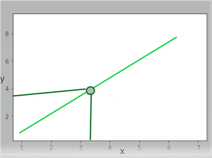
As we all know that the concept of calculus starts with limits, let’s have a quick recap of the limit. We remember a graph with a line that a hole in it, it seemed strange at first, but then it seemed normal, there used to be a notation that used to look like, it is read as the limit of f(x) as x approaches to some number.

In this case, the number is 1. X is coming closer to one, and from the left side of the graph, we can see and record the y values as x comes closer to 1.

The graph is here for a better visualization

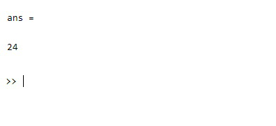
Now let us consider the function f(x)=x^2+x+4, and you want to find out the limit when x approaches 4.  

Example:

Matlab

% MATLAB code for function f(x)=x^2+x+4,
% and find out the limit when x approaches 4
syms x
f = x^2+x+4;
limit(f,x,4)

Output:

 Now let’s take some trigonometric functions, let the function be sin(x)-cos(x)/cos2x when x approaches pi/4.

Example:

Matlab

% MATLAB code for trigonometric functions
% function be sin(x)-cos(x)/cos2x when x = pi/4
syms x

f = sin(x)-cos(X)/cos2x;
limit(f,x,pi/4)

Output:

ans =  -1/√2  

Differentiation in MATLAB

Differentiation is the process of finding the derivative of a function with respect to a variable, derivative means the rate of change of a function with respect to a variable. We applied differentiation to find the velocity rate in Physics and other fields. Derivatives are the functions that tell us the slope of a line tangent to the curve at any point. In dy/dx, the variable y is being differentiated with respect to x. Let’s look at the following graph.

There is a slope and the green line, let us call that secant line, now if we want to find the distance between the two points of the line, we will use the slope formula, that is m=(y2-y1/x2-x1). In this case, the coordinates are (x, f(x)) and (f(x+h),f(x)), the slope will be a difference quotient, given the figure, but this is just an approximation, we don’t need an approximation, we need an exact solution, we need to come closer to x from the start of the secant line, or let’s say, we need to minimize the h, we need h to be zero and when h is zero and the line becomes the tangent of the curve, we take the limit of the difference quotient. 

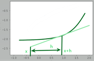
This method of finding derivatives is called finding derivatives when the limit is given. 

Let us see some examples regarding derivatives of algebraic functions. 

Example:

Matlab

% MATLAB code for derivatives
% of algebraic function
syms x
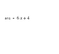
f= 3x^2+4x+5;
diff(f)

Output:

If we want to differentiate exponential functions, then 

Example:

Matlab

% MATLAB code for derivatives
% of algebraic function
syms y
y = exp(x)*tan(x);
diff(y)

Output:

The product rule is used here, that is 

Integration in MATLAB

The integrals, also called anti derivatives, are responsible for finding the area under the curve, the concept of integration can be understood by the following graph

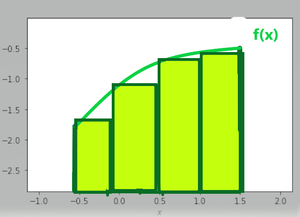
The above graph has a curve, and if we want to find the area under that curve, then an approach is followed here, the curve is filled with rectangles the summation of the rectangles will be  the area of the curve, but the issue is, there’s a lot of blank space, we denote it by Δx, but we still can fill the curve with more rectangles, 

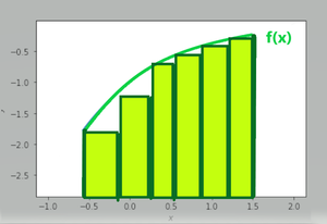
As we can see, the  Δx is really reduced, but to completely eliminate it, we need more rectangle, 

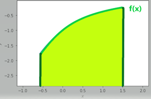
So by filling in enough rectangle or the rectangle’s width approaches zero in width, the Δx becomes dx, and we have our answer. Since we have discussed that integrals are reverse derivatives, the integration of 2x will be x^2, and the differentiation of x^2 will be 2x. Now let’s see some examples of integrals, by the way, an integral is shown or represented by ∫ this symbol.

Let us see how to integrate an algebraic expression in MATLAB

Example:

Matlab

% MATLAB code for integrate
% an algebraic expression
f=@(x)sin(x)+cos(x);
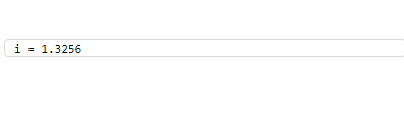
i=integral(f,0,45)

Output:

Let’s see some advanced concepts in Calculus. 

Vector Calculus

Vectors have both quantities magnitude and direction,  it is having magnitude and definitely, it’ll be flowing in some direction, similarly, if we are walking it will be in a particular direction. The concept of vector algebra is highly used in STEM. But why do we need to integrate or differentiate vectors, because when it comes to solving partial differential equations, or fluid flow, or gravitational felids, it is helpful, so if we integrate or differentiate the vector, we integrate the X and Y axis separately.

The Curl and Divergence of a Vector Field

Curl and Divergence, also known as the language of Maxwell’s equations, fluid flow, and more; but to understand them, let us visualize a fluid flowing from somewhere and visualize the electromagnetic field. Now from using the concept of divergence, we can find out the flow of fluid expanding at a given point, divergence is a scalar quantity and not a vector, as it defines the rate of fluid expanding at a point since there is no involvement of the direction, it is a scalar quantity, to find the divergence of a vector field in a 3-dimensional space, we perform a dot product of the partial derivative operator( also caller grad) to the field, mathematically, let F be the vector field in 3-d space and let x,y,z be its co-ordinates, then the divergence of Vector field will be

In the case of positive divergence, the flow is outward, like expanding hot gas, in the case of negative divergence, the case of cool gas being compressed is considered. To visualize this concept, imagine filling some air in a balloon, the balloon will inflate, this is the one example where one can visualize the positive divergence.

Now let’s see how to find the divergence in MATLAB 

Matlab

syms x,y,z

field = [x^2 y^3 z^4];
dimensions= [x y z];
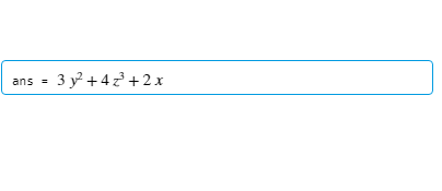
divergence(field, dimensions)

Output:

Now let see about Curl if we need to find the circulation of a vector in 3-d space, then we will use Curl, it is the circulation density at each point of the field. Suppose there is a vector with three dimensions, then the curl of the vector will be

For doing the same in MATLAB,  let us assume V to be the vector field with respect to vector X, both of them having three dimensions. Let V =[x^3+y^3+z, y^3+x^3+z, z^3+x^3+y] and X = [x,y,z].

Matlab

syms x y z

V = [x^3+y^3+z, y^3+x^3+z, z^3+x^3+y];
X = [x y z];
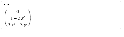
curl(V,X)

Output:

The Curl and Divergence, are also called the language of Maxwell’s Electromagnetic Equations, a set of coupled partial differential equations along with Lorentz Force law, form the fundamentals of Electrodynamics  

Where E is the Electric field, B is the Magnetic Field, H is the Magnetic field strength, and ρ is the charge density. 

The Gradient in MATLAB

The Gradient  is used to define how sharply a  line or slope is rising or falling, the regular method of differentiation gives us the rate of change of a function with just one variable, but what if the function is haver two variables(like f(x,y)), then the concept of gradient comes, suppose the function is

So the gradient of f(x,y) will be the vector form of partial differential with respect to x and y. 

The Geometric meaning of Gradient

Suppose you’re climbing the mountain, and you want to know the path by which you want to reach the top of the mountain fast, or if you just want to contour around the mountain(to be at the same altitude, neither going up nor down), then by use of Gradient, we’ll see that. Let’s see the contour plots here,

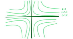
The above figure is a 2-d projection of the Contours in a 3-d plane, so using the concept of gradient and having it plotted gives us the solution of this mountain problem.

Taylor Series

Taylor series is one of the most important theorems in entire calculus. To understand it, let us consider the function e^x at x=0, it is 1, but how do we know when x is 0.2, we will approximate it, there will be an error, but it’ll be a minor one, but when x will be equal to 1.2, the error will be great, let us see the graph below

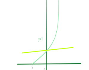
We see a constant function, but by using approximation, we can use a linear approximation, the graph will look something like this

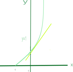
But we can do better than this to approximate, actually, the study of the Taylor series is to take nonpolynomial functions and finding polynomials that approximate near some input, as polynomials are really friendly functions when it comes to integrating or differentiating them, so we need to find the function that spoons best with our exponential graph near x=0. 

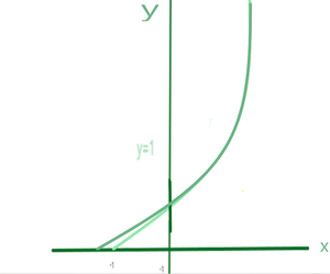
The polynomial function at x=0 is T1= x^4/24 + x^3/6 + x^2/2 + x + 1.

Let us see how to do Taylor approximation in MATLAB

Matlab

syms x
T1 = taylor(exp(x))

Output:

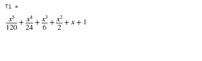
The above code is of the same exponential function shown in the graph, and it will give as output. Taylor’s approximation is used in engineering fields, statistics, physics, and computer science.