Bisecting K-Means Algorithm Introduction

Prerequisite:  K means Clustering – Introduction

K-Means Algorithm has a few limitations which are as follows: 

• It only identifies spherical-shaped clusters i.e it cannot identify, if the clusters are non-spherical or of various sizes and densities.
• It suffers from local minima and has a problem when the data contains outliers.

Bisecting K-Means Algorithm is a modification of the K-Means algorithm. It is a hybrid approach between partitional and hierarchical clustering. It can recognize clusters of any shape and size. This algorithm is convenient because:

• It beats K-Means in entropy measurement.
• When K is big, bisecting k-means is more effective. Every data point in the data collection and k centroids are used in the K-means method for computation. On the other hand, only the data points from one cluster and two centroids are used in each Bisecting stage of Bisecting k-means. As a result, computation time is shortened.
• While k-means is known to yield clusters of varied sizes, bisecting k-means results in clusters of comparable sizes.

Note: Entropy measurement is a measure of the randomness in the data being processed. Example: Flipping a coin. If the entropy of the given data, being processed is high, it is difficult to conclude from that data. 

Example 1 — Say, you walk into a hall consisting of many chairs, and sit on, one of them without observing any other chair in particular or thinking if you could hear the speaker on the stage from the chair you are seated. This kind of approach can be called ‘K-Means’.

Example 2 — Say, you walk into a hall consisting of many chairs. You observe all the chairs and decide which one to occupy, based on various factors like if you could hear the speaker from that position and if the chair is placed near the air conditioner. This kind of approach can be called ‘Bisecting K-means.

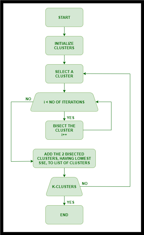
Bisecting K-Means Algorithm:

1. Initialize the list of clusters to accommodate the cluster consisting of all points.
2. repeat
   • Discard a cluster from the list of clusters.
   • { Perform several “trial” bisections of the selected cluster. }
   • for i = 1 to number of trials do
     • Bisect the selected clusters using basic K-means.
   • end for
   • Select the 2 clusters from the bisection with the least total SSE.
3. until Until the list of clusters contain ‘K’ clusters

• The working of this algorithm can be condensed into two steps.
• Firstly, let us assume the number of clusters required at the final stage, ‘K’ = 3 (Any value can be assumed, if not mentioned).

Step 01: 

• All points/objects/instances are put into 1 cluster.

Step 02:

• Apply K-Means (K=3). The cluster ‘GFG’ is split into two clusters ‘GFG1’ and ‘GFG2’. The required number of clusters aren’t obtained yet. Thus, ‘GFG1’ is further split into two (since it has a higher SSE (formula to calculate SSE is explained below))

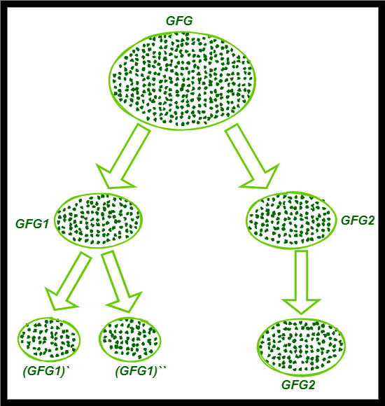
• In the above diagram, as we split the cluster ‘GFG’ into ‘GFG1’ and ‘GFG2’, we calculate the SSE of the two clusters separately using the above formula. The cluster, with the higher SSE, will be split further. The cluster, with the lower SSE, contains lesser errors comparatively, and hence won’t be split further.
• Here, if we get the calculation that the cluster ‘GFG1’ is the one with higher SSE, we split it into (GFG1)` and (GFG1)`. The number of clusters required at the final stage is mentioned as ‘3’, and we obtained 3 clusters.
• If the required number of clusters is not obtained, we should continue splitting until they are produced.

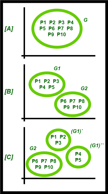
Example:

Consider a cluster ‘G’ = ( P1, P2, P3, P4, P5, P6, P7, P8, P9, P10 ) , consisting of 10 points. K=3 (given)

1. Applying the Bisecting K-Means Algorithm, the cluster ‘G’, as shown in [A]th step is split into two clusters – ‘G1’ and ‘G2’, as shown in [B]th step. The total number of clusters required at the final stage i.e ‘K’=3 (given).
2. Since the required clusters are not obtained yet, we should split one of the two clusters obtained.
3. The cluster with the higher SSE is selected ( since the cluster with a lower SSE is less erroneous). Here, the cluster with higher SSE is cluster ‘G1’. It is split into (G1)` and (G1)“ respectively.
4. Thus, the required number of clusters is obtained.