Binomial Distribution in R Programming
Last Updated :
10 May, 2020
Binomial distribution in R is a probability distribution used in statistics. The binomial distribution is a discrete distribution and has only two outcomes i.e. success or failure. All its trials are independent, the probability of success remains the same and the previous outcome does not affect the next outcome. The outcomes from different trials are independent. Binomial distribution helps us to find the individual probabilities as well as cumulative probabilities over a certain range.
It is also used in many real-life scenarios such as in determining whether a particular lottery ticket has won or not, whether a drug is able to cure a person or not, it can be used to determine the number of heads or tails in a finite number of tosses, for analyzing the outcome of a die, etc.
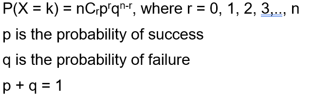
Formula:
Functions for Binomial Distribution
We have four functions for handling binomial distribution in R namely:
- dbinom()
dbinom(k, n, p)
- pbinom()
pbinom(k, n, p)
where n is total number of trials, p is probability of success, k is the value at which the probability has to be found out.
- qbinom()
qbinom(P, n, p)
Where P is the probability, n is the total number of trials and p is the probability of success.
- rbinom()
rbinom(n, N, p)
Where n is numbers of observations, N is the total number of trials, p is the probability of success.
dbinom() Function
This function is used to find probability at a particular value for a data that follows binomial distribution i.e. it finds:
P(X = k)
Syntax:
dbinom(k, n, p)
Example:
dbinom(3, size = 13, prob = 1 / 6)
probabilities <- dbinom(x = c(0:10), size = 10, prob = 1 / 6)
data.frame(x, probs)
plot(0:10, probabilities, type = "l")
|
Output :
> dbinom(3, size = 13, prob = 1/6)
[1] 0.2138454
> probabilities = dbinom(x = c(0:10), size = 10, prob = 1/6)
> data.frame(probabilities)
   probabilities
1   1.615056e-01
2   3.230112e-01
3   2.907100e-01
4   1.550454e-01
5   5.426588e-02
6   1.302381e-02
7   2.170635e-03
8   2.480726e-04
9   1.860544e-05
10  8.269086e-07
11  1.653817e-08
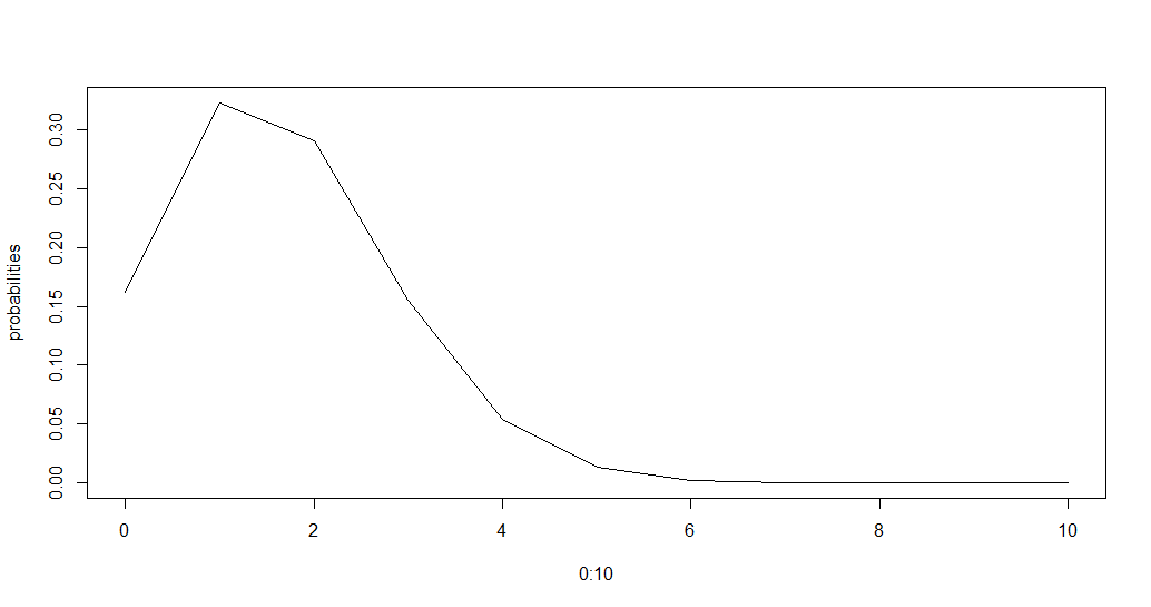
The above piece of code first finds the probability at k=3, then it displays a data frame containing the probability distribution for k from 0 to 10 which in this case is 0 to n.
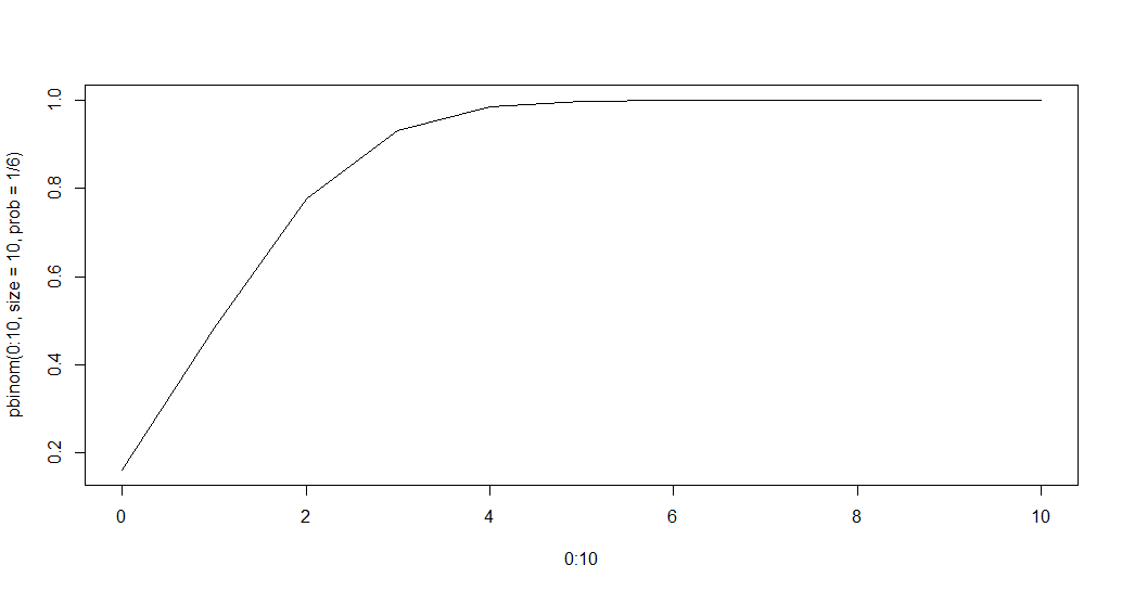
pbinom() Function
The function pbinom() is used to find the cumulative probability of a data following binomial distribution till a given value ie it finds
P(X <= k)
Syntax:
pbinom(k, n, p)
Example:
pbinom(3, size = 13, prob = 1 / 6)
plot(0:10, pbinom(0:10, size = 10, prob = 1 / 6), type = "l")
|
Output :
> pbinom(3, size = 13, prob = 1/6)
[1] 0.8419226
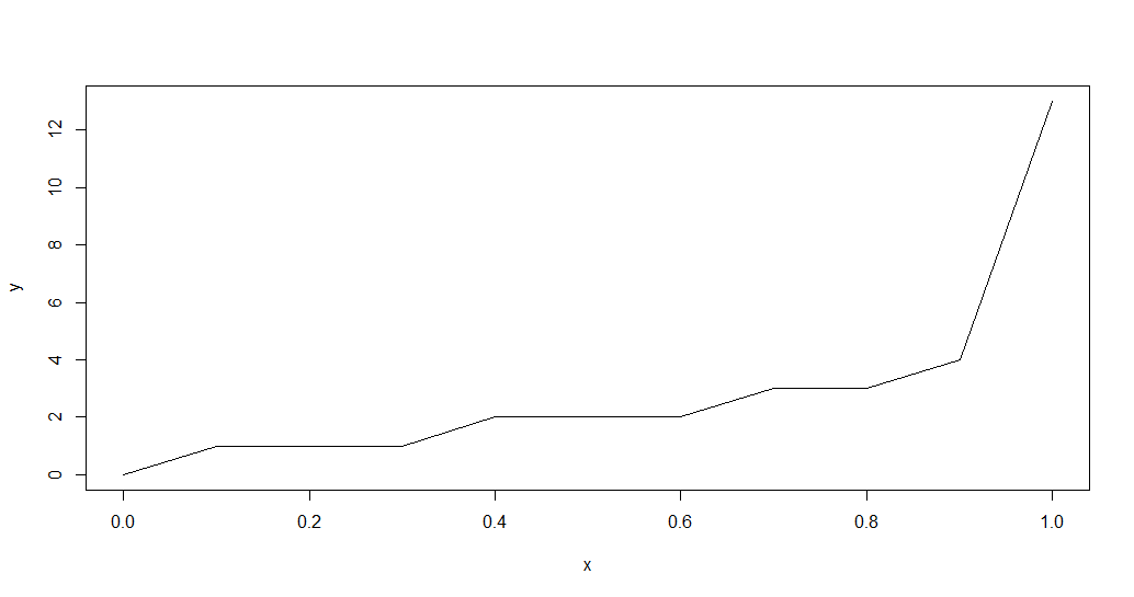
qbinom() Function
This function is used to find the nth quantile, that is if P(x <= k) is given, it finds k.
Syntax:
qbinom(P, n, p)
Example:
qbinom(0.8419226, size = 13, prob = 1 / 6)
x <- seq(0, 1, by = 0.1)
y <- qbinom(x, size = 13, prob = 1 / 6)
plot(x, y, type = 'l')
|
Output :
> qbinom(0.8419226, size = 13, prob = 1/6)
[1] 3
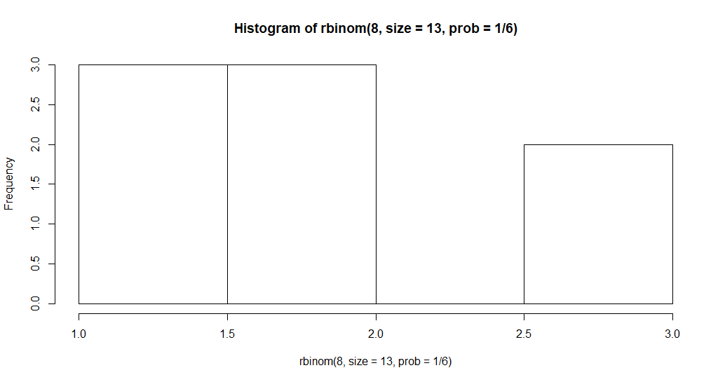
rbinom() Function
This function generates n random variables of a particular probability.
Syntax:
rbinom(n, N, p)
Example:
rbinom(8, size = 13, prob = 1 / 6)
hist(rbinom(8, size = 13, prob = 1 / 6))
|
Output:
> rbinom(8, size = 13, prob = 1/6)
[1] 1 1 2 1 4 0 2 3
Like Article
Suggest improvement
Share your thoughts in the comments
Please Login to comment...