Basic understanding of Jarvis-Patrick Clustering Algorithm
Last Updated :
14 Oct, 2020
Jarvis Patrick Clustering Algorithm is a graph-based clustering technique, that replaces the vicinity between two points with the SNN similarity, which is calculated as described in the SNN Algorithm. A threshold is then accustomed to sparsify this matrix of SNN similarities.
Note: ‘Sparsification’ is a technique where the amount of data, that needs to be processed, is drastically reduced.
SNN Algorithm (Shared Nearest Neighbor similarity) :
- Find the k-nearest neighbors of all points.
- if two points, x and y don’t seem to be among the k-nearest neighbors of each other then
- similarity (x,y)<–0
- else
- similarity (x,y)<– the number of shared neighbors
- end if
JARVIS-PATRICK CLUSTERING ALGORITHM: There are 3 inputs, necessary for the algorithm to work.
- Distance function, to calculate the distance between any two given points.
- ‘k‘, number of the closest neighbors to make note of, while forming clusters.
- ‘kmin‘, the minimum number of shared neighbors for any two given points to be clustered.
The working of the algorithm is as follows:
- The ‘k’ nearest neighbors of all points are found.
- A pair of points are put within the same cluster, if any two points share more than ‘t’ neighbors and also the two points are in each others ‘k’ nearest neighbor list.
- For instance, we might choose the nearest neighbor list of size 30 and put points within the same cluster, if they share more than 15 nearest neighbors.
Example: Jarvis-Patrick clustering of a two-dimensional data set.
- Let us apply, Jarvis-Patrick clustering to the ‘fish’ data-set( as shown in (a) below), to search the clusters (shown in (b) below). The size of the nearest neighbor list was 20, and two points were placed within the identical cluster if they shared a minimum of 10 points. The various clusters are shown by different markers and different shading. The points whose marker is an ‘x’ were classified as noise by Jarvis-Patrick. They are mostly within the transition regions between clusters of assorted density.
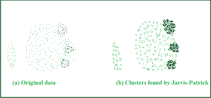
Jarvis-Patrick Clustering of a two-dimensional point set
- Storage requirements of the Jarvis-Patrick clustering algorithm: O (km), since it is not really necessary to store the entire similarity matrix, even initially.
- Basic time complexity of Jarvis-Patrick clustering: O (m^2), since the creation of the k-nearest neighbor list can require the computation of O (m^2) proximity.
- However, for certain types of data, like low-dimensional Euclidean data, e.g., a k-d tree, may be utilized to search the k-nearest neighbors without computing the full similarity matrix, more efficiently. This could reduce the time complexity from O (m^2) to O (m log m).
Strengths :
- Since Jarvis-Patrick clustering is predicated on the notion of SNN similarity, it is good at coping with noise and might handle clusters of assorted sizes, shapes and densities.
- The algorithm works well for high-dimensional data.
- The algorithm is wonderful at finding tight clusters of strongly related objects.
Limitations:
- Jarvis-Patrick clustering defines a cluster as a connected component within the SNN similarity graph. Thus, whether a bunch of objects is split into two clusters or left collectively may rely on a single link. Hence, Jarvis-Patrick clustering is somewhat brittle i.e., it may split true clusters or join clusters that ought to be kept separate,
- In this algorithm, not all objects are clustered. However, these objects will be added to existing clusters, and in some cases, there is no requirement for a full clustering. When put next to other clustering algorithms, choosing the simplest and best values for the parameters may be challenging.
Like Article
Suggest improvement
Share your thoughts in the comments
Please Login to comment...