Introduction to Backtracking – Data Structure and Algorithm Tutorials
Last Updated :
16 Oct, 2023
Backtracking is like trying different paths, and when you hit a dead end, you backtrack to the last choice and try a different route. In this article, we’ll explore the basics of backtracking, how it works, and how it can help solve all sorts of challenging problems. It’s like a method for finding the right way through a complex choices.
What is Backtracking?
Backtracking is a problem-solving algorithmic technique that involves finding a solution incrementally by trying different options and undoing them if they lead to a dead end. It is commonly used in situations where you need to explore multiple possibilities to solve a problem, like searching for a path in a maze or solving puzzles like Sudoku. When a dead end is reached, the algorithm backtracks to the previous decision point and explores a different path until a solution is found or all possibilities have been exhausted.
Backtracking can be defined as a general algorithmic technique that considers searching every possible combination in order to solve a computational problem.
.png)
Introduction to Backtracking
Basic Terminologies
- Candidate: A candidate is a potential choice or element that can be added to the current solution.
- Solution: The solution is a valid and complete configuration that satisfies all problem constraints.
- Partial Solution: A partial solution is an intermediate or incomplete configuration being constructed during the backtracking process.
- Decision Space: The decision space is the set of all possible candidates or choices at each decision point.
- Decision Point: A decision point is a specific step in the algorithm where a candidate is chosen and added to the partial solution.
- Feasible Solution: A feasible solution is a partial or complete solution that adheres to all constraints.
- Dead End: A dead end occurs when a partial solution cannot be extended without violating constraints.
- Backtrack: Backtracking involves undoing previous decisions and returning to a prior decision point.
- Search Space: The search space includes all possible combinations of candidates and choices.
- Optimal Solution: In optimization problems, the optimal solution is the best possible solution.
Types of Backtracking Problems
Problems associated with backtracking can be categorized into 3 categories:
- Decision Problems: Here, we search for a feasible solution.
- Optimization Problems: For this type, we search for the best solution.
- Enumeration Problems: We find set of all possible feasible solutions to the problems of this type.
How does Backtracking works?
As we know backtracking algorithm explores each and every possible path in order to find a valid solution, this exploration of path can be easily understood via given images:
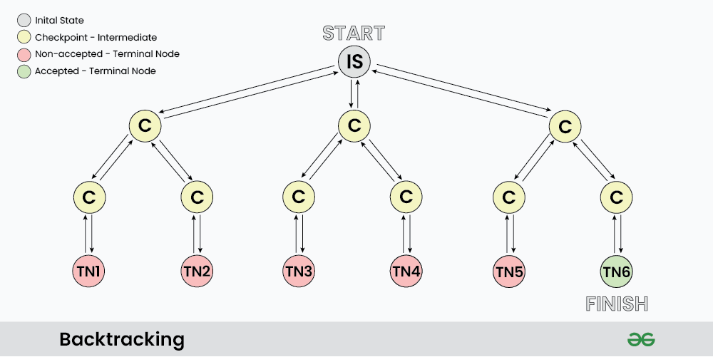
As shown in the image, “IS” represents the Initial State where the recursion call starts to find a valid solution.
C : it represents different Checkpoints for recursive calls
TN: it represents the Terminal Nodes where no further recursive calls can be made, these nodes act as base case of recursion and we determine whether the current solution is valid or not at this state.
At each Checkpoint, our program makes some decisions and move to other checkpoints untill it reaches a terminal Node, after determining whether a solution is valid or not, the program starts to revert back to the checkpoints and try to explore other paths. For example in the above image TN1…TN5 are the terminal node where the solution is not acceptable, while TN6 is the state where we found a valid solution.
The back arrows in the images shows backtracking in actions, where we revert the changes made by some checkpoint.
Determining Backtracking Problems:
Generally every constraint satisfaction problem can be solved using backtracking but, Is it optimal to use backtracking every time? Turns out NO, there are a vast number of problem that can be solved using Greedy or Dynamic programming in logarithmic or polynomial time complexity which is far better than exponential complexity of Backtracking. However many problems still exists that can only be solved using Backtracking.
To understand whether a problem is Backtracking based or not, let us take a simple problem:
Problem: Imagine you have 3 closed boxes, among which 2 are empty and 1 has a gold coin. Your task is to get the gold coin.
Why dynamic programming fails to solve this question: Does opening or closing one box has any effect on the other box? Turns out NO, each and every box is independent of each other and opening/closing state of one box can not determine the transition for other boxes. Hence DP fails.
Why greedy fails to solve this question: Greedy algorithm chooses a local maxima in order to get global maxima, but in this problem each and every box has equal probability of having a gold coin i.e 1/3 hence there is no criteria to make a greedy choice.
Why Backtracking works: As discussed already, backtracking algorithm is simply brute forcing each and every choice, hence we can one by one choose every box to find the gold coin, If a box is found empty we can close it back which acts as a Backtracking step.
Technically, for backtracking problems:
- The algorithm builds a solution by exploring all possible paths created by the choices in the problem, this solution begins with an empty set S={}
- Each choice creates a new sub-tree ‘s’ which we add into are set.
- Now there exist two cases:
- S+s is valid set
- S+s is not valid set
- In case the set is valid then we further make choices and repeat the process until a solution is found, otherwise we backtrack our decision of including ‘s’ and explore other paths until a solution is found or all the possible paths are exhausted.
Pseudocode for Backtracking
The best way to implement backtracking is through recursion, and all backtracking code can be summarised as per the given Pseudocode:
void FIND_SOLUTIONS( parameters):
if (valid solution):
store the solution
Return
for (all choice):
if (valid choice):
APPLY (choice)
FIND_SOLUTIONS (parameters)
BACKTRACK (remove choice)
Return
Complexity Analysis of Backtracking
Since backtracking algorithm is purely brute force therefore in terms of time complexity, it performs very poorly. Generally backtracking can be seen having below mentioned time complexities:
- Exponential (O(K^N))
- Factorial (O(N!))
These complexities are due to the fact that at each state we have multiple choices due to which the number of paths increases and sub-trees expand rapidly.
How Backtracking is different from Recursion?
Recursion and Backtracking are related concepts in computer science and programming, but they are not the same thing. Let’s explore the key differences between them:
|
Recursion does not always need backtracking
|
Backtracking always uses recursion to solve problems
|
|
Solving problems by breaking them into smaller, similar subproblems and solving them recursively.
|
Solving problems with multiple choices and exploring options systematically, backtracking when needed.
|
|
Controlled by function calls and call stack.
|
Managed explicitly with loops and state.
|
|
Applications of Recursion: Tree and Graph Traversal, Towers of Hanoi, Divide and Conquer Algorithms, Merge Sort, Quick Sort, and Binary Search.
|
Application of Backtracking: N Queen problem, Rat in a Maze problem, Knight’s Tour Problem, Sudoku solver, and Graph coloring problems.
|
Applications of Backtracking
- Creating smart bots to play Board Games such as Chess.
- Solving mazes and puzzles such as N-Queen problem.
- Network Routing and Congestion Control.
- Decryption
- Text Justification
Must Do Backtracking Problems
For more practice problems: click here
Like Article
Suggest improvement
Share your thoughts in the comments
Please Login to comment...