Average Cells Based On Multiple Criteria in Excel

An Average is a number expressing the central or typical value in a set of data, in particular the mode, median, or (most commonly) the mean, which is calculated by dividing the sum of the values in the set by their number. The basic formula for the average of n numbers x₁,x₂,……x_n is

A = (x₁ + x₂ ……..x_n)/ n

Excel AVERAGE Function

In Excel, there is an average function for this purpose, but it can be calculated manually using SUM and COUNT functions like this

= SUM(D1:D5)/COUNT(D1:D5)

Where,

SUM: This function is used to find the sum of values in the required range of cells.

COUNT: This function is used to get the count of the required range of cells containing numeric values.

Excel provides a direct function named AVERAGE to calculate the average (or mean) of the numbers in the range specified in the function’s argument. In this function, a maximum of 255 arguments can be given (numbers/cell references/ ranges/ arrays or constants).

Syntax:

= AVERAGE(Num1, [Num2], …)

Where

Num1 [Required]: Provide range, cell references, or the first number for calculating the average.

Num2, … [Optional]: Provide additional numbers or a range of cell references for calculating the average.

Example: AVERAGE(C1:C5)

This will give the average of numeric values in the range C1 to C5.

Note: In the above-mentioned methods, any criteria for calculating the average cannot be mentioned. For this excel provide another function called AVERAGEIF.

Average Cells Based On One Criterion with Average If Function

Excel provides a direct function named AVERAGEIF to calculate the average (or mean) of the numbers in the range specified that meets particular criteria specified in the function’s argument.

Syntax:

= AVERAGEIF(Range_Cells_For_Criteria, Criteria, [Range_Cells_For_Average])

Where,

Range_Cells_For_Criteria [Required]:

Give the range of cells on which criteria are to be tested.

Criteria [Required]:

This is the condition on which to decide the cells to average. The criteria can be given in the form of an expression(logical), text-value or number, or reference to a cell, e.g. 100 or “>100” or “Apple” or A7.

Range_Cells_For_Average [Optional]:

Specify the cells on which the average needs to be calculated. Range_Cells_For_Criteria is used to find the average if it is not included.

Note:

1. An empty cell in average_range is ignored here.
2. Cells in the range that contain TRUE or FALSE are ignored here.
3. If the range is blank, return the #DIV0! Error value.
4. An empty cell in the criteria is treated as 0.

Using Double Quotes (“”) In Criteria

In Excel, the text values are surrounded by double quotations (“), but integers are not, in general. But when numbers are used in criteria(s) with a logical operator, the number and operator must also be wrapped in quotes. 

Examples:

1. To calculate the average of only positive numbers excluding 0 in the range A2 to A6
= AVERAGEIF(A2:A6,”>0″) is correct.
= AVERAGEIF(A2:A6,>0) is incorrect as the logical operator should be included in double quotes.

2. To get the average age (AGE is in column C) of the employees living in the city having id = 1 (CityId is in column D)
= AVERAGEIF(D2:D10, “=1”, C2:C10) is correct
= AVERAGEIF(D2:D10, 1, C2:C10) is also correct as here also D2 to D10 cells will be checked for value 1.

3. To get the average age (AGE is in column C) of the employees living in a city named Mumbai (City is in column B)
= AVERAGEIF(B2:B10, “Mumbai”, C2:C10) is correct 
= AVERAGEIF(B2:B10, Mumbai, C2:C10) is incorrect as text should be included in double quotes.

Example 1: To calculate the average of only positive numbers excluding 0 in the range A2 to A6.

Solution: In this example, a single criterion is given- “>0″. So all the numbers in the range that are greater than 0 come in the criteria. The average will be calculated as

(12.7 + 87.2 + 100) / 3 = 66.66666667

So, the average formula for the above example is

AVERAGEIF(A2:A6,”>0″)

example

Example 2: To get the average age (AGE is in column C) of the employees living in a city named Mumbai (City is in column B).

Solution: Let’s break the example into different parts so that the individual parts can then be substituted in the AVERAGEIF function

• Criteria: “Mumbai”.
• Cells for criteria: B2 to B6.
• Cells for average: C2 to C6 that meet the criteria.

The average age of the employees living in Mumbai

= (65 + 45) /2 = 55

So, the average formula for this example is

AVERAGEIF(B2:B6,”Mumbai”,C2:C6)

example

AVERAGEIFS Function in Excel

The AVERAGEIFS function is used to calculates the arithmetic mean of all cells in a range that meet the specified criteria.

Average Cells Based On Multiple Criterion

Excel provides a direct function named AVERAGEIFS to calculate the average (or mean) of the numbers in the range specified that meets multiple criteria specified in the function’s argument.

Syntax:

AVERAGEIFS(RangeForAverage,RangeForCriteria1,Criteria1,
[RangeForCriteria2, Criteria2],..)

Here

1. RangeForAverage [Required]: Provide the cell range on which the average needs to be computed.
2. RangeForCriteria1: Range on which criteria1 is applied.
3. Criteria 1Criteria 1: The first criteria to apply on the RangeForCriteria1.

AVERAGEIFS Function

Consider the below points to get a clear understanding of how the function works, and avoid errors:

• In the RangeForAverage argument, empty cells, logical values TRUE/FALSE , and text values are ignored. Zero Values are included.
• If criteria is an empty cell, it is treated as a zero value.
• If RangeForAverage doesn’t’ contain a single numeric value, a #DIV/0! error occurs.
• If no cells meet all of the specified criteria, a#DIV/0! error is returned.
• AVERAGEIFS’s criteria may apply to the same range or different ranges.
• Each criteria_range must be of the same size and shape as RangeForAverage, otherwise a #VALUE! error occurs.

Note:

1. All ranges are required along with their criteria.
2. Criteria 1 is required, the rest are optional.

Excel AVERAGEIFS Formula

Let’s understand the AVERAGEIFS formula stepwise:

Pick your Range:

Decide on the range of numbers you want to average. It could be a bunch of sales figure, test scores, or anything else you need an average for.

Set your Criteria:

Think about what conditions your numbers need to meet. Is it sales above a certain amount? Scores from a specific month? These are your criteria.

Follow the Formula Dance:

In the Formula, first tell Excel the range of numbers you want to average. Then, list your c criteria in pairs, where the first is the range to check, and teh second is teh criteria itself. You can have as many pairs as you need.

Odd is the Magic number:

Your AVEARGEIFS Formula should have an odd number of arguments. That means it starts with your average range and then pairs up the criteria ranges and criteria themselves.

Example 1: To calculate the average age of the employees living in Mumbai whose ages are > 50.

Solution: The following criteria are used to solve the problem

• RangeForAverage: C2 to C8.
• Criteria 1: “Mumbai”.
• RangeForCriteria1: B2 to B8.
• Criteria 2: “>50”.
• RangeForCriteria1: C2 to C8.

Here, the average is calculated on the basis of two criteria- Employees living in Mumbai and employees whose Age > 50

AVERAGEIFS(C2:C8,B2:B8,”Mumbai”,C2:C8,”>50″)

example

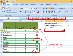
Example 2: To get the average price of the product with Category ID 1 and having a Price greater than Rs 500/-.

Solution: The following criteria will be used for the AVERAGEIF function

• RangeForAverage: C2 to C11.
• Criteria 1: “=1”.
• RangeForCriteria1: B2 to B11.
• Criteria 2: “>500”.
• RangeForCriteria2: C2 to C11.

Here, the average is calculated based on two criteria- Product having Category ID 1 and Price greater than 500

AVERAGEIFSC2:C11,B2:B11,”=1″,C2:C11,”>500″)

example

Using Values From Another Cell

The concatenation of text can be used to use the value from another cell. Concatenation is the process of connecting two or more values to form a text string. There are two ways to concatenation of the strings in Excel

1. Logical & operator can be used.
2. Concatenate function in Excel for concatenation of two texts.

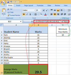
Example: To get average marks (marks are in column B) of passed students having minimum passing marks value contained in cell D2.

Solution: In this example, the logical & operator will be used to concatenate the two conditions for finding the result

• Marks greater than 0.
• Minimum passing marks i.e. 10.

Here, D2 has a value of 10, so the minimum pass marks are 10, the following criteria will be used- “>=”&D2. This will concat “>=” & value contained in cell D2, i.e. 10. After concatenation, the criteria will become “>=10”.

So, in this example

• RangeForAverage- B2 to B12.
• Criteria1- Marks greater than 0.
• RangeForCriteria1- B2 to B12.

The following formula will be used to calculate the average

=AVERAGEIFS(B2:B12,B2:B12,”>=0″&D2)

example

AVERAGEIFS with Wildcard Characters

Excel provides wildcard characters that can be used in the criteria. Some wild cards are

1. * (asterisk): This symbol can be used to represent any number of characters.
2. ? (question mark): This symbol can be used to represent a single character.
3. ~ (tilde): This symbol is used before the above two wild cards and also tilde itself so that when there is a need to match a text containing * or? Or ~, Excel does not treat them as a wildcard. To treat them as normal characters in Excel criteria, the tilde is used before them.

Examples: There are the product names in column A (From A1 to A10) and their respective price in column C.

1. AVERAGEIFS(C2:C11, A:A11, “*a*”): To find the average price of all the products who have character ‘a’ anywhere in their name.
2. AVERAGEIFS(C2:C11, A:A11, “?a*”): To find the average price of all the products that have the second character ‘a’ in their name.
3. AVERAGEIFS(C2:C11, A:A11, “?aree”): To find the average price of all the products that have a single character before ‘aree’ in their name.
4. AVERAGEIFS(C2:C11, A:A11, ” ~*Saree “): To find the average price of all the products that have a name is *Saree.

Example: To find the average price of all the products that have character ‘a’ anywhere in their name.

Solution: In this example

1. Product Saree, Nail Paint, Jeans, and Lehenga contains the character ‘a’ in them.
2. The average prices for these products will be

= (1200+ 100+ 1000+ 5000)/4 = 7300/4 = 1825 

So, the complete formula for calculating the average is as follows

AVERAGEIFS(C2:C11,A2:A11,”*a”)

example

AVERAGE IF between two Values

When you want to find the average of values nestled between two specific points, Excel’s has few examples:

For an Inclusive Range(including boundary Values):

AVERAGEIFS(average_range, criteria_raneg, “>=value1”, criteria_range, “<=value2”)

For an Exclusive Range(excluding boundary values):

AVERAGEIFS(average_range, criteria_range, “>value1”, criteria_range, “<value2”)

In the first formula, the “greater than or equal to “(>=) and “less than or equal to”(<=0 play matchmaker, making sure the boundary values are part of the average party.

For the second formula, the “greater than”(>) and “less than”(<) criteria give a nod to values that sit inside the boundaries but leave out those right on the edges.

These formulas are versatile (work on both scenarios)- when cells to average and the cells to check are in the same column or in two different columns.

Conclusion

Using AVERAGE, it is possible to find average without any criteria. Using AVERAGEIF, the average can be calculated with particular criteria and using AVERAGEIFS, the average can be computed with multiple criteria(s).

FAQs on Average Cells Based On Multiple Criteria

What is “Average Cells Based on Multiple Criteria” in Excel?

“Average Cells Based on Multiple Criteria” is a powerful Excel technique used to calculate the average of cells that meet specific conditions or criteria. This helps you to extract more targeted and meaningful average from your data.

How to calculate the average of cells based on multiple criteria?

You can use the AVERAGEIFS function to calculate the average of cells based on multiple cells. This Function allows you to specify multiple conditions or criteria that the data must meet to be included in the calculation.

Is there a limit to the number of criteria I can use with AVERAGEIFS?

No, there is no specific limit to the number of criteria you can with the AVERAGEIFS Function. You can include as many criteria as needed to refine your average calculation.

What are the alternatives to AVERAGEIFS for averaging cells based on multiple criteria?

You can also use the SUMPRODUCT Function to average cells based on multiple criteria that include dates, text, and numeric values. It provides the flexibility to work with various data types simultaneously.