Apache Pig Installation on Windows and Case Study

Apache Pig is a data manipulation tool that is built over Hadoop’s MapReduce. Pig provides us with a scripting language for easier and faster data manipulation. This scripting language is called Pig Latin.

Apache Pig scripts can be executed in 3 ways as follows:

• Using Grunt Shell (Interactive Mode) – Write the commands in the grunt shell and get the output there itself using the DUMP command.
• Using Pig Scripts (Batch Mode) – Write the pig latin commands in a single file with .pig extension and execute the script on the prompt.
• Using User-Defined Functions (Embedded Mode) – Write your own Functions on languages like Java and then use them in the scripts.

Pig Installation:

Before proceeding you need to make sure that you have all these pre-requisites as follows.

1. Hadoop Ecosystem installed on your system and all the four components i.e. DataNode, NameNode, ResourceManager, TaskManager are working. If any one of them randomly shuts down then you need to fix that before proceeding.
2. 7-Zip is required to extract the .tar.gz files in windows.

Let’s take a look at How to install Pig version (0.17.0) on Windows as follows.

Step 1: Download the Pig version 0.17.0 tar file from the official Apache pig site. Navigate to the website https://downloads.apache.org/pig/latest/. Download the file ‘pig-0.17.0.tar.gz’ from the website. 

Then extract this tar file using 7-Zip tool (use 7-Zip for faster extraction.  First we extract the .tar.gz file by right-clicking on it and clicking on ‘7-Zip → Extract Here’. Then we extract the .tar file in the same way). To have the same paths as you can see in the diagram then you need to extract in the C: drive.

Step 2: Add the path variables of PIG_HOME and PIG_HOME\bin

Click the Windows Button and in the search bar type ‘Environment Variables’. Then click on the ‘Edit the system environment variables’.

Then Click on ‘Environment Variables’ on the bottom of the tab. In the newly opened tab click on the ‘New’ button in the user variables section.

After hitting new Add the following values in the fields.

Variable Name  -  PIG_HOME
Variable value -  C:\pig-0.17.0

All the path to the extracted pig folder in the Variable Value field. I extracted it in the ‘C’ directory. And then click OK.

Now click on the Path variable in the System variables. This will open a new tab. Then click the ‘New’ button. And add the value C:\pig-0.17.0\bin in the text box. Then hit OK until all tabs have closed.

Step 3: Correcting the Pig Command File

Find file ‘pig.cmd’ in the bin folder of the pig file ( C:\pig-0.17.0\bin)

set HADOOP_BIN_PATH = %HADOOP_HOME%\bin

Find the line:

set HADOOP_BIN_PATH=%HADOOP_HOME%\bin 

Replace this line by:

set HADOOP_BIN_PATH=%HADOOP_HOME%\libexec 

And save this file. We are finally here. Now you are all set to start exploring Pig and it’s environment.

There are 2 Ways of Invoking the grunt shell:

Local Mode: All the files are installed, accessed, and run in the local machine itself. No need to use HDFS. The command for running Pig in local mode is as follows. 

pig -x local

MapReduce Mode: The files are all present on the HDFS . We need to load this data to process it. The command for running Pig in MapReduce/HDFS Mode is as follows. 

pig -x mapreduce

Apache PIG CASE STUDY:

1. Download the dataset containing the Agriculture related data about crops in various regions and their area and produce. The link for dataset –https://www.kaggle.com/abhinand05/crop-production-in-india The dataset contains 7 columns namely as follows.

State_Name : chararray ; 
District_Name : chararray ;  
Crop_Year : int ; 
Season : chararray ; 
Crop : chararray ;  
Area : int ; 
Production : int

No of rows: 246092 
No of columns: 7

2. Enter pig local mode using

grunt > pig -x local

3. Load the dataset in the local mode

grunt > agriculture= LOAD 'F:/csv files/crop_production.csv' using PigStorage (',') 
        as ( State_Name:chararray , District_Name:chararray , Crop_Year:int , 
        Season:chararray , Crop:chararray , Area:int , Production:int ) ;

4. Dump and describe the data set agriculture using

grunt > dump agriculture;
grunt > describe agriculture;

5. Executing the PIG queries in local mode

You can follow these written queries to analyze the dataset using the various functions and operators in PIG. You need to follow all the above steps before proceeding.

Query 1: Grouping All Records State wise.

This command will group all the records by the column State_Name.

grunt > statewisecrop = GROUP agriculture BY State_Name;
grunt > DUMP statewisecrop;
grunt > DESCRIBE statewisecrop;

Now store the result of the query in a CSV file for better understanding. We have to mention the name of the object and the path where it needs to be stored.  

pathname -> 'F:/csv files/statewiseoutput'
grunt > STORE statewisecrop INTO ‘F:/csv files/statewiseoutput’;

The output will be in a file named ‘part-r-00000’ which needs to be renamed as ‘part-r-00000.csv’ to be opened in the Excel format and to make it readable. You will find this file in the path that we have mentioned in the above query. In my case it was in the path ‘F:/csv files/statewiseoutput/’.

The output file will look something like this:

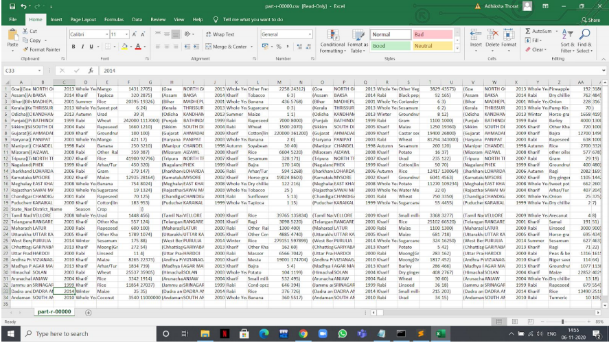
CSV file of output of query 1

You can also check the raw file by opening the command prompt in administrator mode and write the following command as follows.

 C:\Users\Adhiksha\ > Head -2 ‘F:\csv files\statewiseoutput\part-r-00000.csv’;

This command returns the top 2 records of the state-wise output result file. Looks something like this.

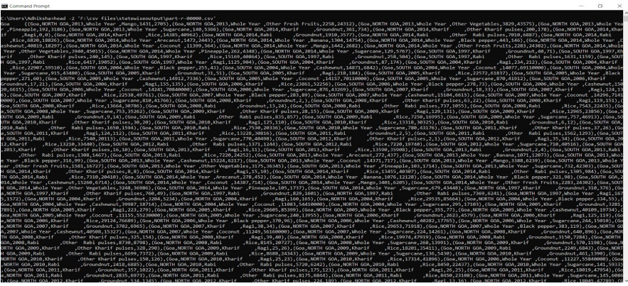
Output of query number 1

Query 2: Generate Total Crop wise Production and Area

In the above query, we need to group by Crop type and then find the SUM of their Productions and Area.

grunt > cropinfo = FOREACH( GROUP agriculture BY Crop )
GENERATE group AS Crop, SUM(agriculture.Area) as AreaPerCrop , 
SUM(agriculture.Production) as ProductionPerCrop;
grunt > DESCRIBE cropinfo;

grunt > STORE cropinfo INTO ‘F:/csv files/cropinfooutput’;

The output will be in a file named ‘part-r-00000’ which needs to be renamed as ‘part-r-00000.csv’ to be opened in the Excel format and to make it readable.

You can check the csv output by opening the command prompt in administrator mode and running the command as follows.

C:\Users > cat ‘F:/csv files/cropinfooutput/part-r-00000.csv’

This will return all the output on the command prompt. You can see that we have three columns in the output. 

Output:

Crop , 
AreaperCrop , 
ProductionPerCrop.

Query 3: The majority of crops are grown in a Season and in which year.

In this query, we need to group the crops by season and order them alphabetically. Also, this will tell us which crops are found in a season and with year.

grunt > seasonalcrops = FOREACH (GROUP agriculture by Season ){
                        order_crops = ORDER agriculture BY Crop ASC;
                        GENERATE group AS Season , order_crops.(Crop) AS Crops;
                        };

grunt > DESCRIBE seasonalcrops;

grunt > STORE seasonalcrops INTO ‘F:/csv files/seasonaloutput;

The output will be in a file named ‘part-r-00000’ which needs to be renamed as ‘part-r-00000.csv’ to be opened in the Excel format and to make it readable. You can check the csv output by opening the command prompt in administrator mode and running the command as follows.

 C:\Users > cat ‘F:/csv files/seasonaloutput/part-r-00000.csv’

You can check the output from the ‘part-r-00000.csv’ by opening the file. You can see all the distinct seasons in the first row followed by all the crops and their years of production.

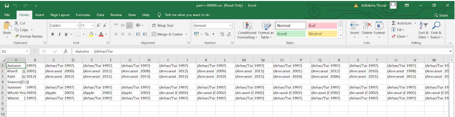
Output of this query number 3

Query 4: Average crop production in each district after the year 2000.

First, we need to group by district name and then find the average of the total crop production but only after the year 2000.

grunt > averagecrops = FOREACH (GROUP agriculture by District_Name){
                       after_year = FILTER agriculture BY Crop_Year>2000;
                       GENERATE group AS District_Name , AVG(after_year.(Production)) AS
                       AvgProd;
                       };

 grunt > DESCRIBE averagecrops;

 grunt > STORE averagecrops INTO ‘F:/csv files/averagecrops;

You can check the output from the ‘part-r-00000.csv’ by opening the file. This file will contain two columns. The first one has all distinct district names and the second one will have the average production of all crops in each district after the year 2000.

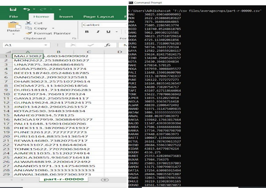
Output of the query number 4

Query 5: Highest produced crops and details from each State.

First, we need to group the input by the state name. Then iterate through each grouped record and then find the TOP 1 record with the highest Production from each state.

grunt > top_agri= GROUP agriculture BY State_Name;
grunt > data_top = FOREACH top_agri{
                   top = TOP(1, 6 , agriculture);
                   GENERATE top as Record;
                   }

grunt > DESCRIBE cropinfo;

grunt > STORE averagecrops INTO ‘F:/csv files/averagecrops;

You can check the output from the ‘part-r-00000.csv’ by opening the file. This file contains records from each unique state who are having the highest Production amount. Read above and follow the steps to create ‘part-r-00000.csv’. You can check the csv output by opening the command prompt in administrator mode and running the command:

C:\Users > cat ‘F:/csv files/top1prod/part-r-00000.csv’