An introduction to MultiLabel classification

One of the most used capabilities of supervised machine learning techniques is for classifying content, employed in many contexts like telling if a given restaurant review is positive or negative or inferring if there is a cat or a dog on an image. This task may be divided into three domains, binary classification, multiclass classification, and multilabel classification. In this article, we are going to explain those types of classification and why they are different from each other and show a real-life scenario where the multilabel classification can be employed.

The differences between the types of classifications

• Binary classification:
  It is used when there are only two distinct classes and the data we want to classify belongs exclusively to one of those classes, e.g. to classify if a post about a given product as positive or negative;
• Multiclass classification: It is used when there are three or more classes and the data we want to classify belongs exclusively to one of those classes, e.g. to classify if a semaphore on an image is red, yellow or green;
• Multilabel classification:
  It is used when there are two or more classes and the data we want to classify may belong to none of the classes or all of them at the same time, e.g. to classify which traffic signs are contained on an image.

Real-world multilabel classification scenario
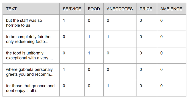
The problem we will be addressing in this tutorial is extracting the aspect of restaurant reviews from twitter. In this context, the author of the text may mention none or all aspects of a preset list, in our case this list is formed by five aspects: service, food, anecdotes, price, and ambience. To train the model we are going to use a dataset originally proposed for a competition in 2014 at the International Workshop on Semantic Evaluation, it is known as SemEval-2014 and contains data about the aspects in the text and its respective polarities, for this tutorial we are only using the data about the aspects, more information about the original competition and its data may be found on their  site .

For the sake of simplicity in this tutorial, the original XML file was converted into a CSV file which will be available on GitHub with the full code. Each row is formed by the text and the aspects contained on it, the presence or absence of those aspects is represented by 1 and 0 respectively, the image below shows how the table looks like.

The first thing we need to do is importing the required libraries, all the of them are in the code snippet below if you are familiar with machine learning you will probably recognize some of those.

Code: Importing Libraries

import pandas as pd
import numpy as np
from sklearn.model_selection import train_test_split
from sklearn.feature_extraction.text import TfidfVectorizer
from skmultilearn.adapt import MLkNN
from sklearn.metrics import hamming_loss, accuracy_score

After that, we have to import the texts and split them properly to train the model, however, the raw text itself does not make a lot a sense to machine learning algorithms, for this reason, we have to represent them differently, there are many different forms to represent text, here we will be using a simple but very powerful technique called TF-IDF which stands for Term Frequency – Inverse Document Frequency, in a nutshell, it is used to represent the importance of each word inside a text corpus, you may find more details about TF-IDF on this  incredible article . In the code below we’ll assign the set of texts to X and the aspects contained on each text to y, to convert the data from row text to TF-IDF we’ll create an instance of the class TfidfVectorizer, using the function fit to provide the full set of texts to it so later we can use this class to convert the split sets, and finally, we’ll split the data between train and test data using 70% of the data to train and keeping the rest to test the final model and convert each of those sets using the function transform from the instance of TfidfVectorizer we have created earlier.
Code:

aspects_df = pd.read_csv('semeval2014.csv')
X = aspects_df["text"]
y = np.asarray(aspects_df[aspects_df.columns[1:]])

# initializing TfidfVectorizer
vetorizar = TfidfVectorizer(max_features=3000, max_df=0.85)
# fitting the tf-idf on the given data
vetorizar.fit(X)

# splitting the data to training and testing data set
X_train, X_test, y_train, y_test = train_test_split(X, y, test_size=0.30, random_state=42)

# transforming the data
X_train_tfidf = vetorizar.transform(X_train)
X_test_tfidf = vetorizar.transform(X_test)

Now everything is set up so we can instantiate the model and train it! Several approaches can be used to perform a multilabel classification, the one employed here will be MLKnn, which is an adaptation of the famous Knn algorithm, just like its predecessor MLKnn infers the classes of the target based on the distance between it and the data from the training base but assuming it may belong to none or all the classes.
Code:

# using Multi-label kNN classifier
mlknn_classifier = MLkNN()
mlknn_classifier.fit(X_train_tfidf, y_train)

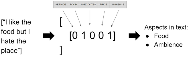
Once the model is trained we can run a little test and see it working with any sentence, I’ll be using the sentence “I like the food but I hate the place” but feel free to use any sentences you like. As we did to the train and test data we need to convert the vector of new sentences to TF-IDF and after that use the function  predict from the model instance which will provide us with a sparse matrix that can be converted to an array with the function toarrayreturning an array of arrays where each element on each array infers the presence of an aspect as shown on image 2.

Code:

new_sentences = ["I like the food but I hate the place"]
new_sentence_tfidf = vetorizar.transform(new_sentences)

predicted_sentences = mlknn_classifier.predict(new_sentence_tfidf)
print(predicted_sentences.toarray())

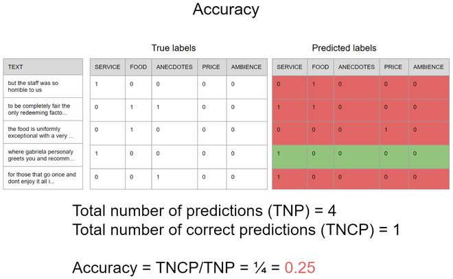
Now, we have to do one of the most important parts of the machine learning pipeline, the testing. At this part, there are some significant differences from multiclass problems, for instance, we can not use accuracy in the same way because one single prediction infers many classes at the same time, as in the hypothetic scenario shown in the image 3, note that when using accuracy only the predictions that are exactly equal to the true labels are considered a correct prediction, thus the accuracy is 0.25 which means that if you are trying to predict the aspects of 100 sentences in only 25 of them the presence and absence of all aspects would be predicted correctly at the same time.

On the other hand, there is a more appropriate metric that can be used to measure how good the model is predicting the presence of each aspect independently, this metric is called hamming loss, and it is equal to the number of incorrect prediction divided by the total number of predictions where the output of the model may contain one or more predictions, the following image that uses the same scenario of the last example illustrates how it works,  it is important to note that unlikely accuracy in hamming loss the smaller the result is the better is the model. Thus the hamming loss, in this case, is 0.32 which means that if you are trying to predict the aspects of 100 sentences the model will predict incorrectly about 32% of the independent aspects.

Although the second metric seems to be more suited for problems like this is important to keep in mind that all machine learning problems are different from each other, therefore each of them may combine a different set of metrics to better understand the model’s performance, as always, there is no silver bullet. To use those we are going to use the metrics module from sklearn, which takes the prediction performed by the model using the test data and compares with the true labels.

Code:

predicted = mlknn_classifier.predict(X_test_tfidf)

print(accuracy_score(y_test, predicted))
print(hamming_loss(y_test, predicted))

So now if everything is right with accuracy near 0.47 and a hamming loss near to 0.16!