Amplitude Modulation based on Depth of Modulation(Modulation Factor) using GNU Octave

Modulation in communication systems is a widely used process in which characteristics like amplitude, frequency, or phase angle of a high-frequency carrier wave is varied according to the instantaneous value of the low-frequency message signal.

Amplitude modulation is a modulation technique utilized in electronic communication, most ordinarily for transmitting data by means of a carrier wave. In amplitude modulation, the amplitude that is the signal quality of the carrier wave differs with respect to that of the message signal being transmitted.

There are mainly three types of modulation techniques: Amplitude Modulation, Frequency Modulation, and Phase Modulation.

In this article, we are going to discuss how to generate the Amplitude Modulated waveforms using GNU Octave.

GNU Octave is an open-source software that supports high-level programming language. It is similar to MATLAB in terms of writing the program/code for performing various mathematical operations or plots. You can learn how to perform basic operations on Octave from here.

Amplitude modulation of a sine wave can be generated using Octave with the following programs: 

Assigning all the required parameters:

MATLAB

% time sampling where Step Size = 0.001
t = 0:0.001:1

% frequency of input or modulating signal
fm = 10

% frequency of output or modulated signal
fc = 100

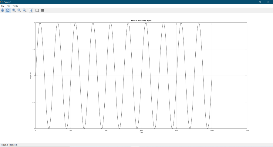
Program to visualize the Modulating Signal:

MATLAB

% Input or Modulating Signal
input_signal = sin(2 * pi * fm * t)
plot(input_signal,'k') % 'k' gives black colour plot

xlabel('Time')
ylabel('Amplitude')
title('Input or Modulating Signal')

Output:

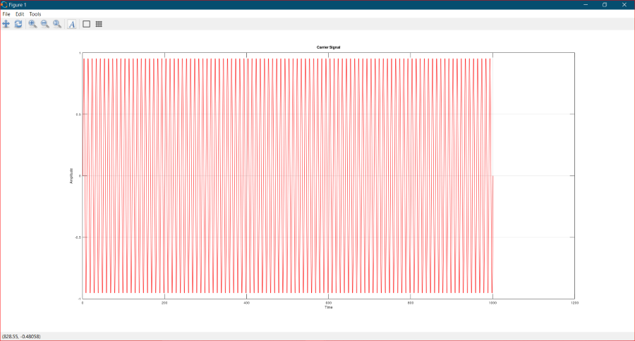
Program to visualize the Carrier Signal:

MATLAB

% Carrier Signal
carrier_signal = sin(2 * pi * fc *t)
plot(carrier_signal,'r') % 'r' gives red colour plot

xlabel('Time')
ylabel('Amplitude')
title('Carrier Signal')

Output:

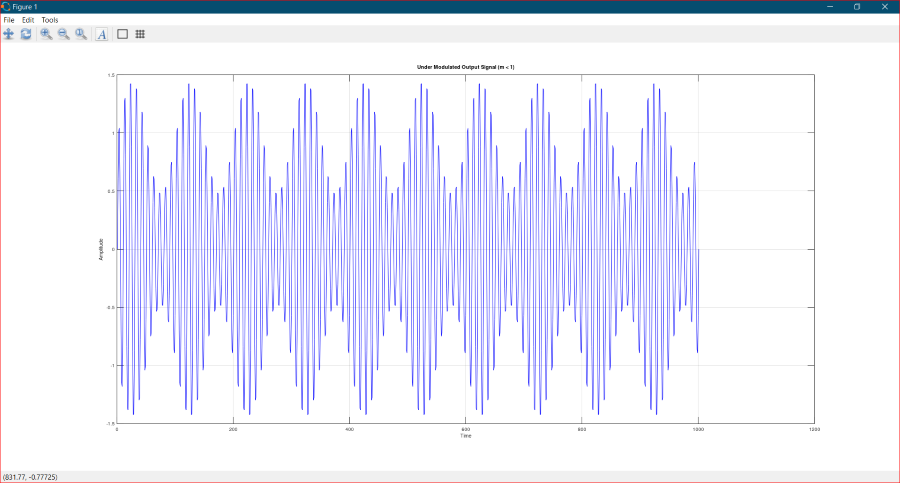
There are three different cases of Amplitude Modulation depending upon the value of modulation factor also known as depth of modulation (m). The modulation factor can be defined as the ratio of the difference between the maximum and minimum amplitudes of the modulated signal to the sum of these amplitudes.

• Under Modulation (m < 1)

MATLAB

% Output or Amplitude Modulated Signal (Under Modulated)
m = 0.5 % modulation factor (m < 1)
under_modulated_signal = (1 + m * sin(2 * pi * fm *t)) .* sin(2 * pi * fc * t)
plot(under_modulated_signal,'b') % 'b' gives blue colour plot

xlabel('Time')
ylabel('Amplitude')
title('Under Modulated Output Signal (m < 1)')

Output:

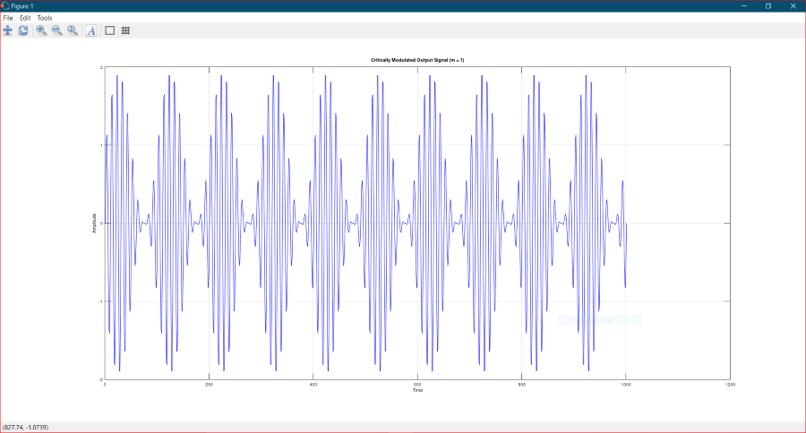
• Critical or Full Modulation (m = 1)

MATLAB

% Output or Amplitude Modulated Signal (Fully or Critically Modulated)
m = 1.0 % modulation factor (m = 1)
fully_modulated_signal = (1 + m * sin(2 * pi * fm *t)) .* sin(2 * pi * fc * t)
plot(fully_modulated_signal,'b') % 'b' gives blue colour plot

xlabel('Time')
ylabel('Amplitude')
title('Critically Modulated Output Signal (m = 1)')

Output:

• Over Modulation (m > 1)

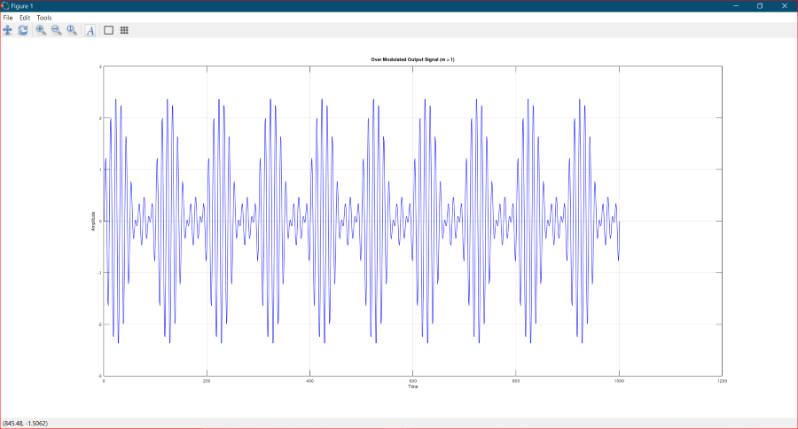
MATLAB

% Output or Amplitude Modulated Signal (Over Modulated)
m = 1.5 % modulation factor (m > 1)
over_modulated_signal = (1 + m * sin(2 * pi * fm *t)) .* sin(2 * pi * fc * t)
plot(over_modulated_signal,'b') % 'b' gives blue colour plot

xlabel('Time')
ylabel('Amplitude')
title('Over Modulated Output Signal (m > 1)')

Output:

If you want to implement Amplitude Modulation using MATLAB, then please take guidance from here.