A Practical approach to Simple Linear Regression using R

Simple Linear Regression is a statistical method that allows us to summarize and study relationships between two continuous (quantitative) variables. One variable denoted x is regarded as an independent variable and other one denoted y is regarded as a dependent variable. It is assumed that the two variables are linearly related. Hence, we try to find a linear function that predicts the response value (y) as accurately as possible as a function of the feature or independent variable (x). The simplest form of the regression equation with one dependent and one independent variable is defined by the formula:

y = c + b * x where: y = estimated dependent variable score, c = constant, b = regression coefficient, and x = score on the independent variable.

Dependent Variable is also called as outcome variable, criterion variable, endogenous variable, or regressand. Independent Variable is also called as exogenous variables, predictor variables, or regressors. The overall idea of regression is to examine two things –

1. Does a set of predictor variables do a good job in predicting an outcome (dependent) variable?
2. Which variables, in particular, are significant predictors of the outcome variable, and in what way do they–indicated by the magnitude and sign of the beta estimates–impact the outcome variable?

These simple linear regression estimates are used to explain the relationship between one dependent variable and one independent variable. 
Now, here we would implement the linear regression approach to one of our datasets. The dataset that we are using here is the salary dataset of some organization that decides its salary based on the number of years the employee has worked in the organization. So, we need to find out if there is any relation between the number of years the employee has worked and the salary he/she gets. Then we are going to test that the model that we have made on the training dataset is working fine with the test dataset or not.

Step #1: The first thing that you need to do is to download the dataset from here. Save the downloaded dataset in your system so that it is easy to fetch when required.

Step #2: The next is to open the R studio since we are going to implement the regression in the R environment. Step #3: Now in this step we are going to deal with the whole operation that we are going to perform in the R studio. Commands with their brief explanation are as follows – Loading the Dataset – The first step is to set the working directory. Working directory means the directory in which you are currently working. setwd() is used to set the working directory.

setwd("C:/Users/hp/Desktop")

Now we are going to load the dataset to the R studio. In this case, we have a CSV (comma separated values) file, so we are going to use the read.csv() to load the Salary_Data.csv dataset to the R environment. Also, we are going to assign the dataset to a variable and here suppose let’s take the name of the variable to be as raw_data. 

R

raw_data <- read.csv("Salary_Data.csv")

Now, to view the dataset on the R studio, use name of the variable to which we have loaded the dataset in the previous step.

raw_data

Step #4: Splitting the Dataset. Now we are going to split the dataset into the training dataset and the test dataset.

Training data, also called AI training data, training set, training dataset, or learning set — is the information used to train an algorithm. The training data includes both input data and the corresponding expected output. Based on this “ground truth” data, the algorithm can learn how to apply technologies such as neural networks, to learn and produce complex results, so that it can make accurate decisions when later presented with new data. Testing data, on the other hand, includes only input data, not the corresponding expected output. The testing data is used to assess how well your algorithm was trained, and to estimate model properties.

For doing the splitting, we need to install the caTools package and import the caTools library.

install.packages('caTools')
library(caTools)

Now, we will set the seed. When we will split the whole dataset into the training dataset and the test dataset, then this seed will enable us to make the same partitions in the datasets.

set.seed(123)

Now, after setting the seed, we will finally split the dataset. In general, it is recommended to split the dataset in the ratio of 3:1. That is 75% of the original dataset would be our training dataset and 25% of the original dataset would be our test dataset. But, here in this dataset, we are having only 30 rows. So, it is more appropriate to allow 20 rows(i.e. 2/3 part) to the training dataset and 10 rows(i.e. 1/3 part) to the test dataset.

split = sample.split(raw_data$Salary, SplitRatio = 2/3)

Here sample.split() is the function that splits the original dataset. The first argument of this function denotes on the basis of which column we want to split our dataset. Here, we have done the splitting on the basis of Salary column. SplitRatio specifies the part that would be allocated to the training dataset. Now, the subset with the split = TRUE will be assigned to the training dataset and the subset with the split = FALSE will be assigned to the test dataset.

training_set <- subset(raw_data, split == TRUE)
test_set <- subset(raw_data, split == FALSE)

Step #5: Fitting the Linear Simple Regression to the Training Dataset. Now, we will make a linear regression model that will fit our training dataset. lm() function is used to do so. lm() is used to fit linear models. It can be used to carry out regression, single stratum analysis of variance, and analysis of covariance.

regressor = lm(formula = Salary ~ YearsExperience, data = training_set)

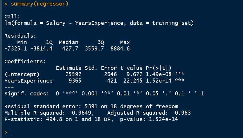
Basically, there are a number of arguments for the lm() function but here we are not going to use all of them. The first argument specifies the formula that we want to use to set our linear model. Here, we have used Years of Experience as an independent variable to predict the dependent variable that is the Salary. The second argument specifies which dataset we want to feed to the regressor to build our model. We are going to use the training dataset to feed the regressor. After training our model on the training dataset, it is the time to analyze our model. To do so, write the following command in the R console:

summary(regressor)

Step #6: Predicting the best set results Now, it is time to predict the test set results based on the model that we have made on the training dataset. predict() function is used to do so. The first argument we have passed in the function is the model. Here, the model is regressor. The second argument is newdata that specifies which dataset we want to implement our trained model on and predict the results of the new dataset. Here, we have taken the test_set on which we want to implement our model.

y_pred = predict(regressor, newdata = test_set)

Step #7: Visualizing the Training Set results We are going to visualize the training set results. For doing this we are going to use the ggplot2 library. ggplot2 is a system for declaratively creating graphics, based on The Grammar of Graphics. You provide the data, tell ggplot2 how to map variables to aesthetics, what graphical primitives to use, and it takes care of the details. 

R

library(ggplot2)

ggplot() +
  geom_point(aes(x = training_set$YearsExperience,
                 y = training_set$Salary), colour = 'red') +
  geom_line(aes(x = training_set$YearsExperience,
                y = predict(regressor, newdata = training_set)),
               colour = 'blue') +
  ggtitle('Salary vs Experience (Training Set)') +
           xlab('Years of Experience') +
           ylab('Salary')

Output: 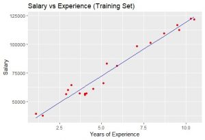The blue-colored straight line in the graph represents the regressor that we have made from the training dataset. Since we are working with simple linear regression, therefore, the straight line is obtained. Also, the red-colored dots represent the actual training dataset. Although, we did not accurately predict the results the model that we have trained was close enough to reach accuracy.   Step #8: Visualising the Test Set Results As we have done for visualizing the training dataset, similarly we can do it to visualize the test dataset also. 

R

library(ggplot2)
ggplot() +
  geom_point(aes(x = test_set$YearsExperience,
                 y = test_set$Salary),
                colour = 'red') +
  geom_line(aes(x = training_set$YearsExperience,
                y = predict(regressor, newdata = training_set)),
                colour = 'blue') +
  ggtitle('Salary vs Experience (Test Set)') +
  xlab('Years of Experience') +
  ylab('Salary')

Output: 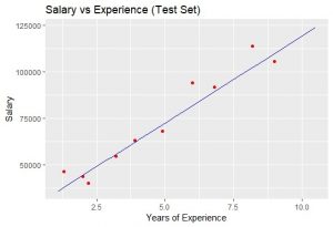Let’s see the complete code for both R and Python – 

R

# Simple Linear Regression

# Importing the dataset
dataset = read.csv('Salary_Data.csv')

# Splitting the dataset into the Training set and Test set
install.packages('caTools')
library(caTools)
set.seed(123)

split = sample.split(dataset$Salary, SplitRatio = 2/3)
training_set = subset(dataset, split == TRUE)
test_set = subset(dataset, split == FALSE)

# Fitting Simple Linear Regression to the Training set
regressor = lm(formula = Salary ~ YearsExperience,
data = training_set)

# Predicting the Test set results
y_pred = predict(regressor, newdata = test_set)

# Visualising the Training set results
library(ggplot2)
ggplot() +
geom_point(aes(x = training_set$YearsExperience,
              y = training_set$Salary),
              colour = 'red') +
geom_line(aes(x = training_set$YearsExperience,
              y = predict(regressor, newdata = training_set)),
              colour = 'blue') +
ggtitle('Salary vs Experience (Training set)') +
xlab('Years of experience') +
ylab('Salary')

# Visualising the Test set results
library(ggplot2)
ggplot() +
geom_point(aes(x = test_set$YearsExperience, y = test_set$Salary),
colour = 'red') +
geom_line(aes(x = training_set$YearsExperience,
              y = predict(regressor, newdata = training_set)),
colour = 'blue') +
ggtitle('Salary vs Experience (Test set)') +
xlab('Years of experience') +
ylab('Salary')

Python

# Simple Linear Regression

# Importing the libraries
import numpy as np
import matplotlib.pyplot as plt
import pandas as pd

# Importing the dataset
dataset = pd.read_csv('Salary_Data.csv')
X = dataset.iloc[:, :-1].values
y = dataset.iloc[:, 1].values

# Splitting the dataset into the Training set and Test set
from sklearn.cross_validation import train_test_split
X_train, X_test, y_train, y_test = train_test_split(
            X, y, test_size = 1/3, random_state = 0)

# Fitting Simple Linear Regression to the Training set
from sklearn.linear_model import LinearRegression
regressor = LinearRegression()
regressor.fit(X_train, y_train)

# Predicting the Test set results
y_pred = regressor.predict(X_test)

# Visualising the Training set results
plt.scatter(X_train, y_train, color = 'red')
plt.plot(X_train, regressor.predict(X_train), color = 'blue')
plt.title('Salary vs Experience (Training set)')
plt.xlabel('Years of Experience')
plt.ylabel('Salary')
plt.show()

# Visualising the Test set results
plt.scatter(X_test, y_test, color = 'red')
plt.plot(X_train, regressor.predict(X_train), color = 'blue')
plt.title('Salary vs Experience (Test set)')
plt.xlabel('Years of Experience')
plt.ylabel('Salary')
plt.show()