2k Factorial Design in R

The R programming language is used for statistical data analysis and machine learning, where the system is trained with a large dataset to analyze, organize and use the calculations to predict and perform tasks based on a similar data format.

Data Visualization plays an important role in R. There are many formats like Box Plots, Histograms, and Barplots in R but for Factorial Design we need to understand the interaction plot.

• The interaction plot is specially used in R to represent the interaction between two independent factors on a particular dataset. The interaction plot function takes in three variables only, the two factors and one dataset.

ANOVA Table

ANOVA (Analysis of Variance) table is a way to present the results of a statistical test used to compare the means of multiple groups. The ANOVA test is used to determine whether there is a significant difference in the means of two or more groups.

An ANOVA table typically includes several rows and columns of information. Some common elements that an ANOVA table may include are:

• Source: This column lists the different sources of variation in the data. For example, in a one-way ANOVA, the source of variation would be the different groups being compared. In a two-way ANOVA, there would be two sources of variation: the first factor and the second factor.
• df: This column lists the degrees of freedom for each source of variation. The degree of freedom (df) is the number of values that are free to vary after the constraints of the problem has been accounted for.
• Sum of Squares (SS): This column lists the sum of squares (SS) for each source of variation. The sum of squares is a measure of the total variability in the data, and it is used to calculate the mean square (MS) and the F-ratio.
• Mean Square (MS): This column lists the mean square (MS) for each source of variation. The mean square is calculated by dividing the sum of squares by the degrees of freedom (MS = SS/df).
• F-ratio: This column lists the F-ratio for each source of variation. The F-ratio is calculated by dividing the mean square for a given source of variation by the mean square for the error term (F = MS / MSerror).
• p-value: This column lists the p-value for each source of variation. The p-value is the probability of obtaining an F-ratio as large or larger than the one computed from the data, assuming that the null hypothesis (i.e., no significant difference between the means) is true.

The results of the ANOVA test are usually considered statistically significant if the p-value is less than the significance level of the test (for example, 0.05). In such a case, you can conclude that at least one of the group means is different from the others. However, it’s important to keep in mind that ANOVA is an omnibus test, which only tells you that there is a difference somewhere, but not where.

2^K  Factorial Design

• The 2^K Factorial Design builds a statistical overview for K factors comprising of 2 levels – High and Low (+ and -). The factors can be quantitative (amount) or qualitative (concentration) of the variables. 
• It is used to identify the factors which have a significant effect on a response variable (given dataset) and to determine the nature of those effects.

Uses of 2^K Factorial Design

1. Ecologists use factorial design to study the effect of multiple environmental factors (for example light intensity, temperature, humidity) on plant growth or the study of different pesticides on an ecosystem.
2. Market researchers use factorial designs to determine the most effective marketing strategy for a product. For example, it can be used to study the interactions between different advertising messages, promotions, and pricing strategies to determine the most effective combination for increasing sales.
3. In manufacturing, a factorial design can be used to determine the optimal levels of factors such as temperature, pressure, and speed that produce the highest-quality product.

Factorial Design for 2²

Here we will deal with 2 factors/variables say A and B. Number of runs will be = 4. Hence the combinations will be { 1, a, b, ab } among which two will be  -ve and two +ve.

Factors		Combination	Exp. 1	Exp. 2	Total
A	B
–	–	A -ve , B -ve	10	20	30
+	–	A +ve , B -ve	40	30	70
–	+	A -ve , B +ve	25	50	75
+	+	A +ve , B +ve	60	70	130

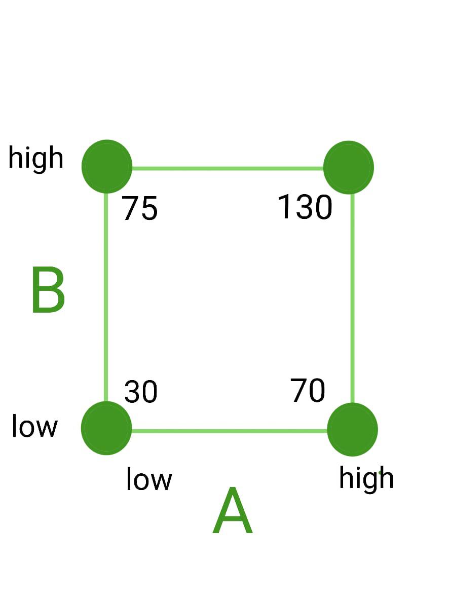
2²  factorial representation

Steps to Represent 2² Factorial Design

Create/Read a csv dataset based on 2 factors each containing two levels along with a response column. You can prepare the table in R using the following syntax :

R

dataset <- data.frame(factor1 = (levels),
                      factor2 = (levels),
                      response = (values))

Assign the factors and response to some variables to further use the variables for the interaction plot.

R

var1 = data$factor1
var2 = data$factor2
response_var = data$response

Use the factors and response to create the ANOVA Table.

R

model <- aov(response ~ factor1*factor2)

If the p-value associated with the factor is less than 0.05, this means the factor has a statistically significant effect on response. Now you can plot the interaction plot.

R

interaction(var1, var2,
            response_var)

QUESTION :

Design an interaction plot in R with 22 factorial designs for the “Deposition of copper covering during Electrolysis” using the following factors.

• A – Electroplating Rate, levels are 40% and 60%.
• B – Deposition Time, levels are less and more

The response variables are the thickness of copper plating in micrometers.

Combinations	Electroplating_Rate	Deposition_Time
(1)	40%	less
a	60%	more
b	60%	less
ab	60%	more

R

#Create a vector column for thickness
thickness<-c(rnorm(15, 6, 4), rnorm(15, 5, 3),
             rnorm(15, 10, 5), rnorm(15,3,1))

#Create the factors
Electroplating_Rate <- c(rep("40%",15),
                         rep("60%",15),
                         rep("60%",15),
                         rep("40%",15))

Deposition_Time <- c(rep("more",30),
                     rep("less",30),
                     rep("more",30),
                     rep("less",30))

#Merge the data into a dataset 'data'
data<- data.frame(Electroplating_Rate,
                  Deposition_Time,
                  thickness)

#Assign the factors into variables
A = data$Electroplating_Rate
B = data$Deposition_Time
Z = data$thickness

result <-aov(Z ~ A*B)

#Plot the anova table
anova(result)

#Plot the interaction plot
interaction.plot(A, B, Z,
                 xlab = "Deposition Time",
                 ylab = "Thickness")

Output:

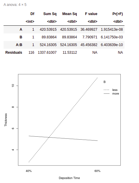
Interaction plot for the ANOVA

Factorial Design for 2³

We will have 3 factors say A, B, and C. Then, we will get 8 runs and the combinations will be { (1), a, b, c, ab, ac, bc, abc}  among which four will be  -ve and four +ve. Similarly, we can get k factors for high and low labels in 2 variable Factorial Designs.

Conclusion

The 2^K factorial designs are particularly useful when the number of factors and their interactions is relatively small, and they are especially powerful when the interactions between factors are suspected to be important. This kind of design allows the analysis of all the possible combinations of factors and interactions, making it possible to identify the main effects of each factor and their interactions and help to identify a good set of parameters for optimization or further experimentation. The significance of combinations decreases after k = 2. The factorial design process in statistics can only be used in equal distribution of labels, i.e. k/2 positive and k/2 negative.